



Two readings of five percent
On 24 July the ECB published the third-quarter round of its Survey of Professional Forecasters. Among much else, the panel attaches a probability of 5.4% to negative euro-area GDP growth over the year to the first quarter of 2027.
In July 2008 the same survey, asking the same question about the year to 2009Q1, produced 5.0%. Growth over that year came in at −5.7%.
Each forecast in this piece is dated to the target quarter it concerns, but was formed roughly two quarters earlier at the one-year horizon. The distinction matters, because the question here is what the panel could have known at the time, not whether its distributions resemble revised data after the fact — asked of a record that contains three episodes of negative annual growth — the events the survey’s question actually defines, which are not the same object as a dated recession chronology. Outcomes are measured on today’s GDP vintage except where real-time releases are cited. A disclosure before the record: I work at the Central Bank of Ireland and in the ESRB Secretariat; this piece is written in a personal capacity, on public data only, and the full statement sits at the end.
The whole distribution
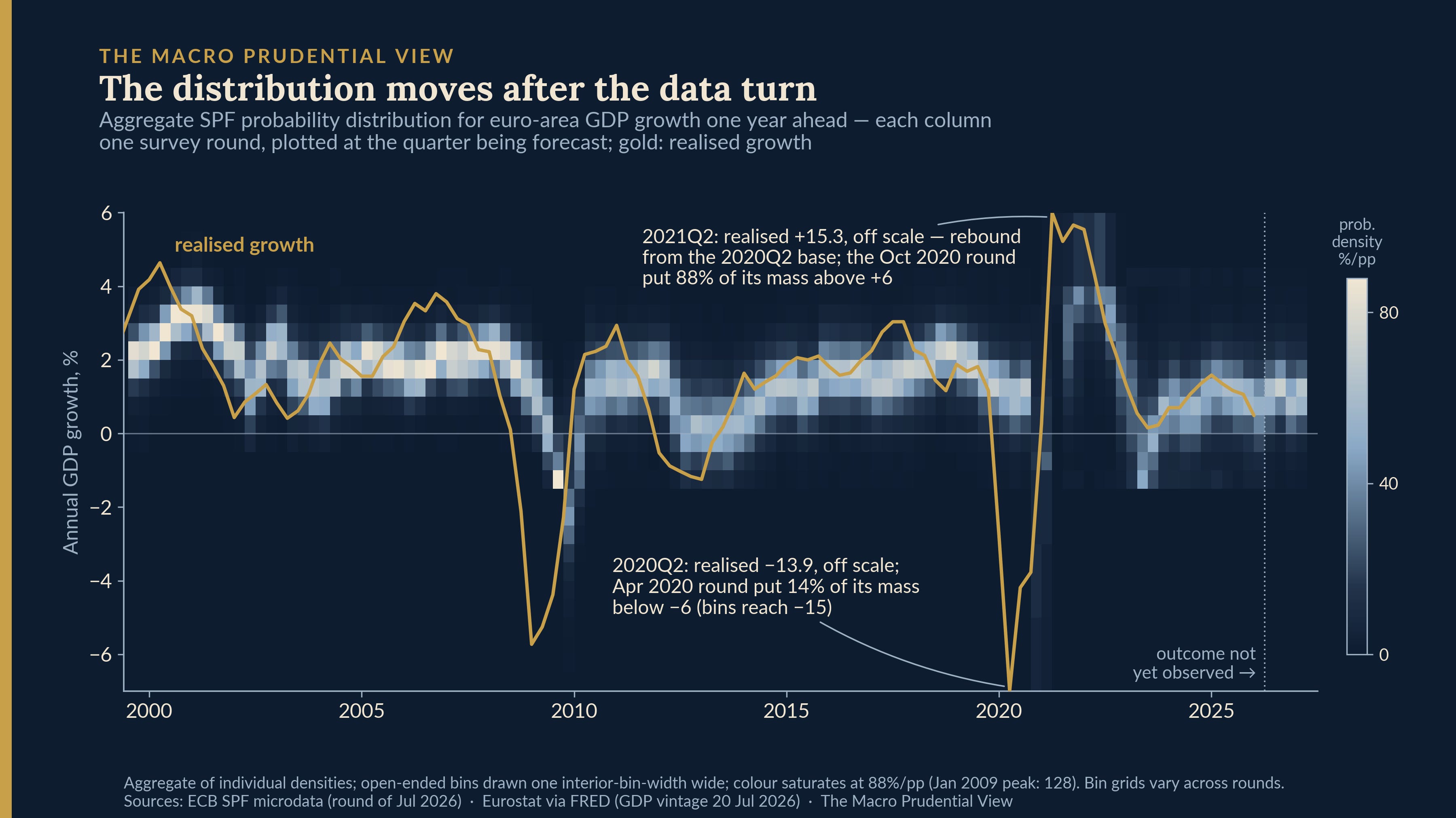
The mechanics briefly, because every caveat in this piece lives in them. Respondents attach probabilities to growth bins — half a percentage point wide in normal times, two points in the COVID-era grid — alongside their point forecasts. I rescale each usable density to sum to one and average across respondents with equal weights, the ECB’s own convention; between 24 and 58 densities survive that filter per round at the one-year horizon. Stacked across 111 rounds, the result is Figure 1: in the major episodes, the distribution shifts materially only after weakness is visible in the information available to respondents. The one emphatic early call is the post-lockdown rebound — 88% of the October 2020 round’s mass above +6% for 2021Q2, which delivered +15.3% — and it was aided by a base effect already embedded in the observed collapse, which makes it weak evidence that the survey can anticipate a downturn nobody has yet seen in the data.
One number in the survey’s favour before anything critical. On a Brier score for the probability of negative growth, the survey scores 0.095 against 0.121 for a constant benchmark set at the sample’s unconditional frequency and 0.132 for an expanding-window climatology using only information available at each origin; the ranking is unchanged excluding the 2020–21 reversal, though a paired bootstrap on the differential does not separate it cleanly from zero (method notes). That gain does not establish early-warning value: a Brier score rewards probability accuracy across all quarters, whereas the macroprudential question is whether the density adds enough information before rare, persistent downside states. Everything that follows is about where the survey’s information sits — in time, and in the distribution.
How to read the charts. A survey round is the forecast origin; fieldwork for the 2008Q3 round, for example, ran from 16 to 23 July 2008. Each round carries a rolling one-year target (annual growth to a quarter roughly two quarters beyond the round, defined as one calendar year beyond the latest available data) and a two-year target roughly six quarters out. Charts are indexed by target quarter, so each forecast sits at the outcome it concerns; the round that produced it, and what it could know, are stated in the annotations. Outcomes are measured on the current GDP vintage (20 July 2026) except where real-time releases are cited.
The warning arrives late
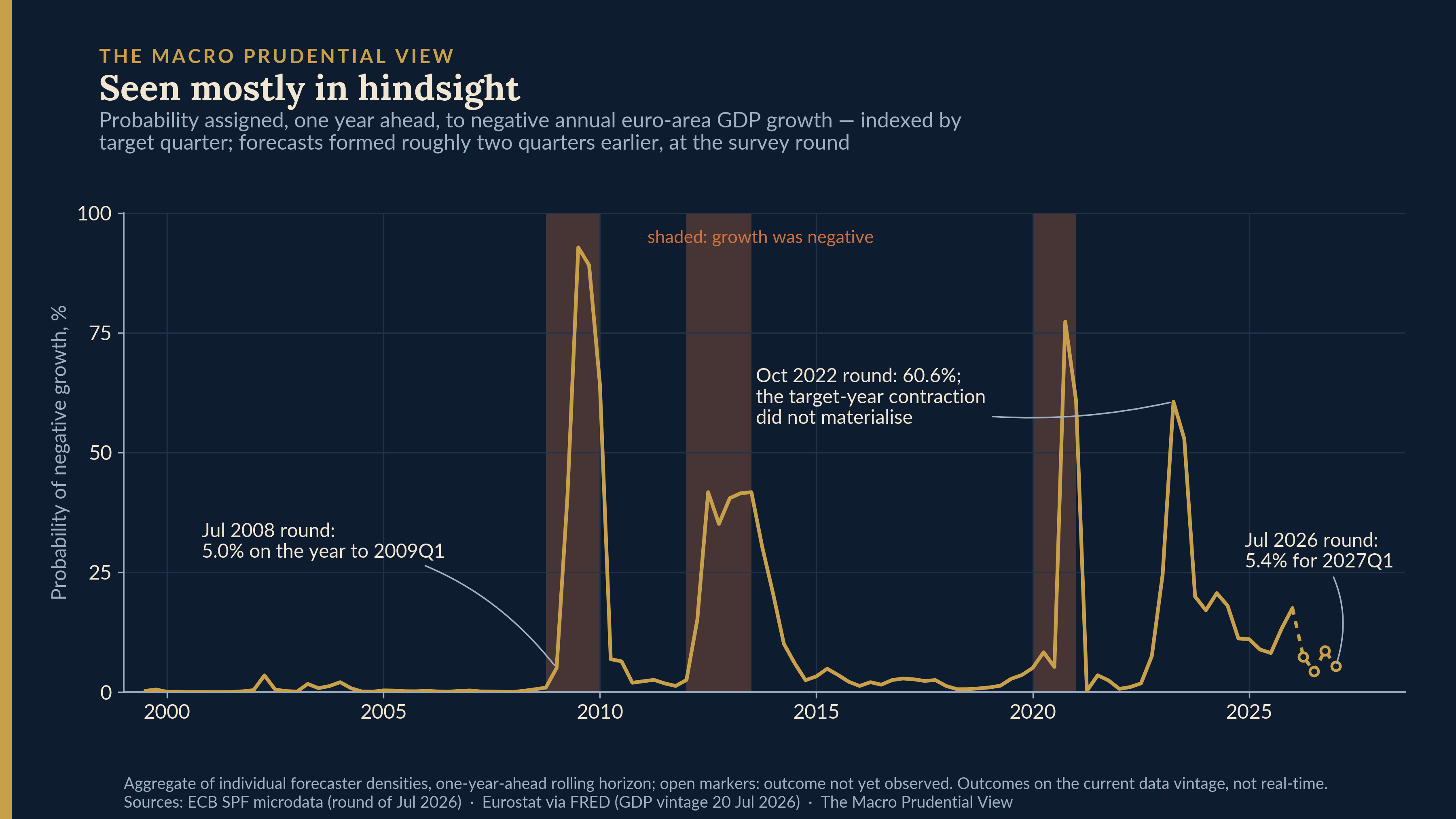
The record across the three recessions reads as follows. July 2008: 5.0% — with published national accounts covering only the first quarter of 2008; Eurostat’s first estimate showing the euro area contracting arrived weeks after fieldwork closed, and even that release put annual growth at +1.4%. October 2008: 40.8%. Two things reached the panel in between. Eurostat’s August flash showed the euro area contracting on the quarter for the first time, though annual growth in that release was still +1.4%; and Lehman Brothers filed on 15 September. No third-quarter national-accounts print existed yet. The repricing followed a financial collapse and a first contraction print together, not a downturn visible in the annual data the forecast concerned. January 2009: 92.8%, after recessionary data had become unmistakable, but while the eventual depth remained far beyond the distribution’s centre. The consensus repriced hard, but not before the year it was forecasting had begun, and it still understated the depth. The 2011–13 recession is the harder case, because it arrived gradually and was debated extensively in real time: the survey’s probability never exceeded 41.7% across six consecutive quarters of negative annual growth. The magnitudes matter for reading that number: outcomes ran between −0.2% and −1.3%, and a 40% probability attached to a mild contraction is not obviously miscalibrated. What the densities did not do is move their centre: the mean of the distribution stayed positive in every one of those rounds, falling from +1.5% to +0.2% but never crossing zero, while the outcomes it was forecasting were negative throughout. October 2019 put 8.3% on the year to 2020Q2, which realised at −13.9%; the pandemic stays in every headline number below and is labelled for what it is, an extreme exogenous shock with little plausible pre-event predictability.
Then the other direction. The sample’s highest one-year probability of negative annual growth — 60.6%, in the October 2022 round, for the year to 2023Q2 — was the largest ex-ante probability in the record not followed by the event, an outcome to which the forecast itself assigned meaningful probability. Revisions could in principle have erased a contraction the forecasters correctly saw. They did not: growth over the year to 2023Q2 was positive in the initial Eurostat release (+0.6%), the subsequent estimate (+0.5%), and today’s vintage (+0.55%). Quarterly growth through late 2023 was weak on every vintage, but the negative annual-growth event to which the probability referred never occurred.
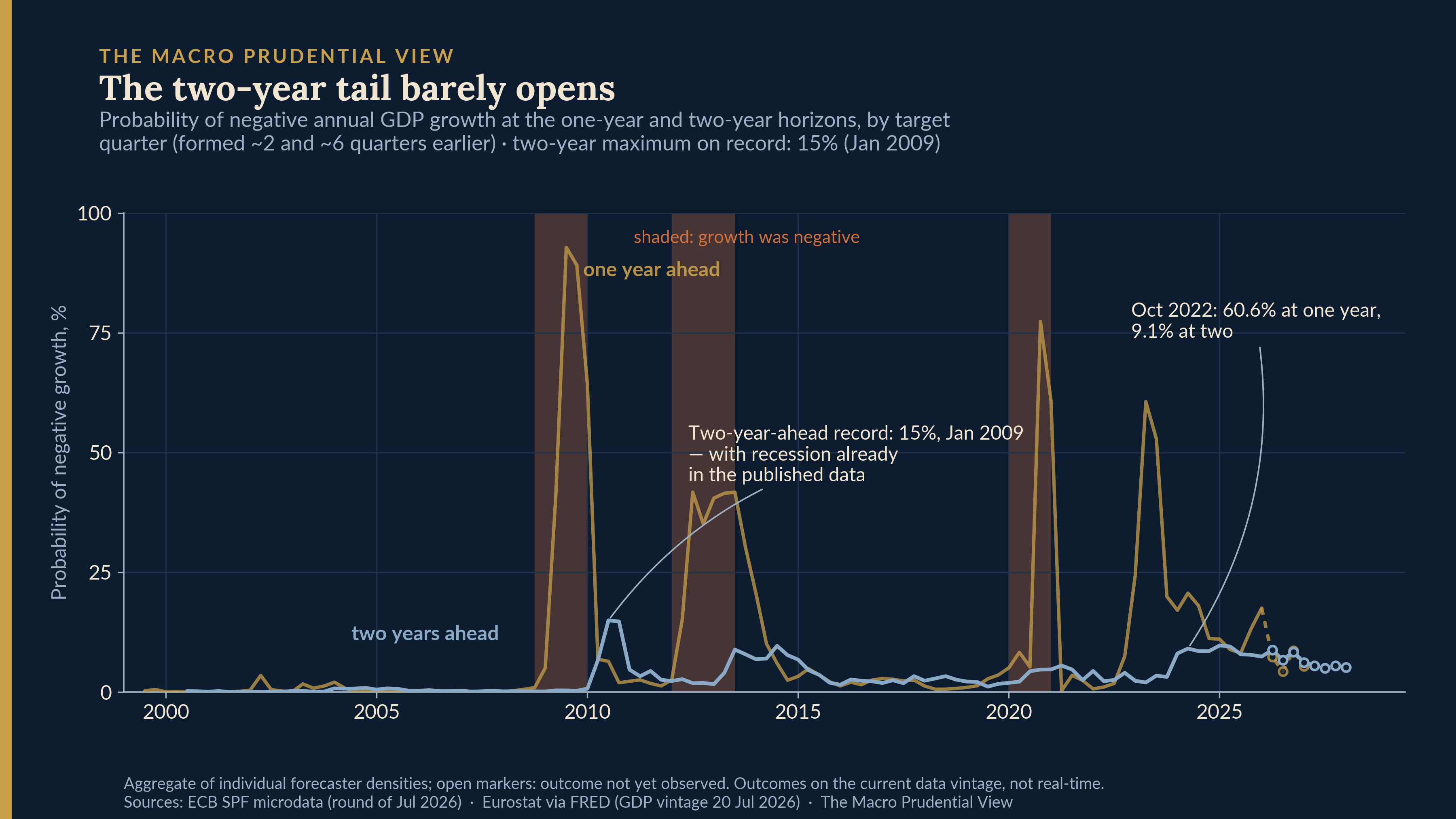
The horizon result completes the picture. At two years the series never opens: its 27-year maximum is 15.0%, set in January 2009, when the recession was already in the published data. In October 2022 the same forecasters who put 60.6% on a negative outcome one year out put 9.1% two years out — not one shock seen at two distances, since the targets are different years and a panel expecting a short contraction followed by recovery would produce exactly that split. What the two-year series establishes is a full-sample property: across 27 years and three downturns, it never opened, whatever the state of the world at the time of asking. For the probability of negative growth at one year, in the downturns this record contains, the tail is a nowcast.
Coverage, honestly bounded
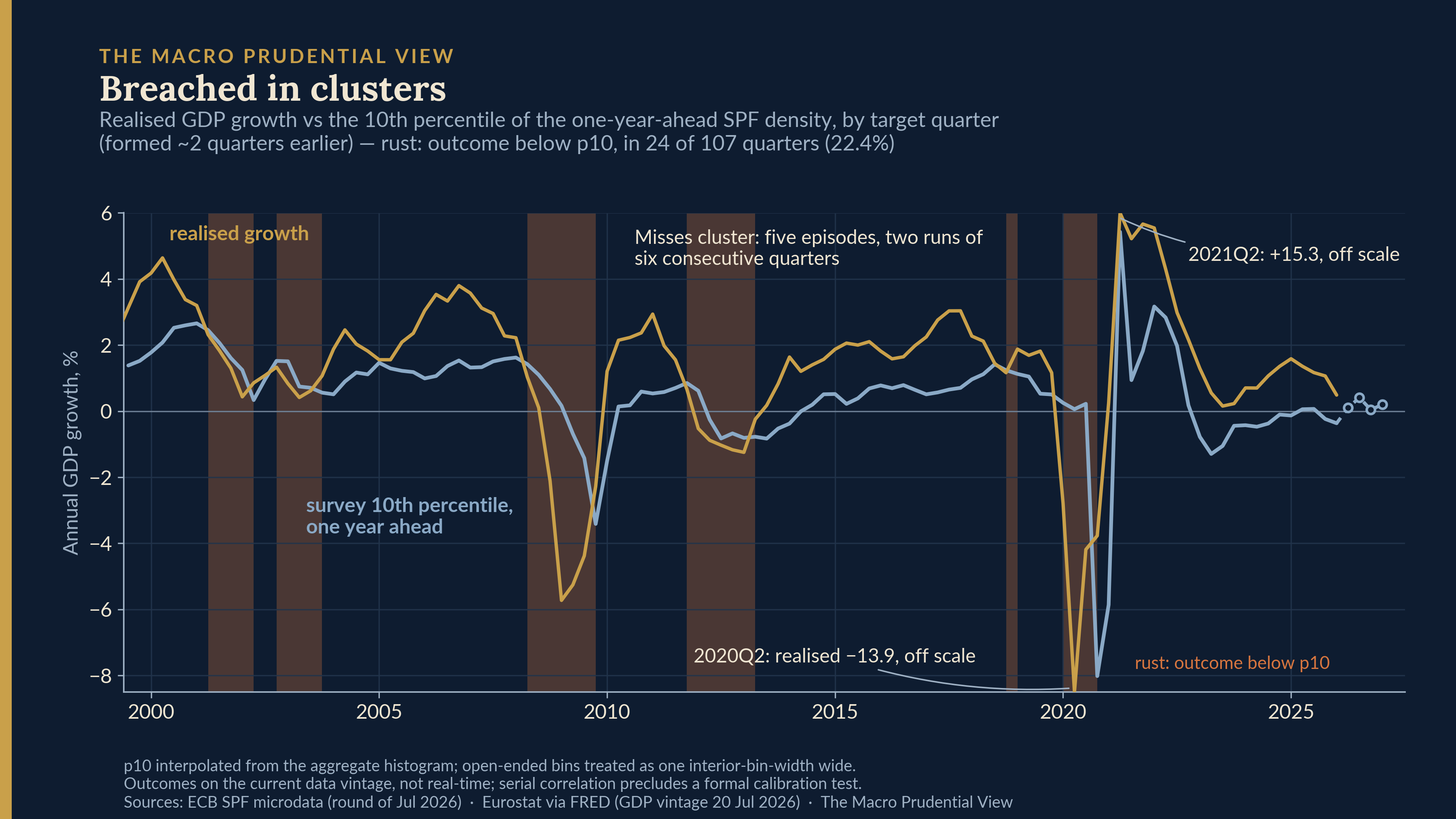
Realised growth fell below the survey’s one-year 10th percentile in 24 of 107 realised target quarters; excluding the four 2020 targets, 21 of 103. Inference has to respect the dependence first: overlapping annual windows make consecutive breaches dependent by construction, some clustering is mechanically induced by that overlap alone, and the effective sample is closer to the number of downturn episodes than to 107. A moving-block bootstrap puts a 95% interval of roughly 10% to 38% around the 22.4% point estimate — the interval excludes neither calibration nor coverage far worse than nominal. What the sample does locate is where the misses sit: in the downturn episodes, twice in runs of six consecutive quarters, rather than scattered through normal times. Because overlap mechanically induces dependence, this is evidence of an episode pattern, not a formal estimate of state-conditional coverage.
Conditioning on the survey’s own probabilities gives a more useful description than the raw rate:
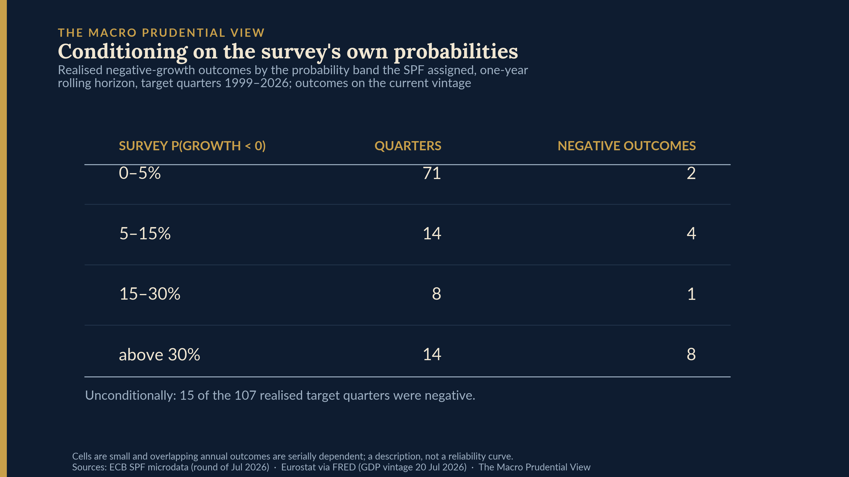
The 5–15% cell contains four negative outcomes in fourteen observations — suggestive, and far too small to define a stable risk band. The relationship is non-monotonic in the middle bands, largely because elevated pessimism persisted after the 2011–13 downturn and again after the 2022 episode. And the 0–5% row, which looks consistent with calibration on frequency, contains a sting: its two events were the onset quarters of the two cyclical downturns, the years to 2008Q4 and to 2012Q1. Two of the 24 breaches are marginal — 2003Q3 by nine basis points, 2018Q4 by seven — and all of this is measured against today’s vintage rather than the data forecasters faced. Frequency calibration is not magnitude protection.
Two episodes, and what the panel knew
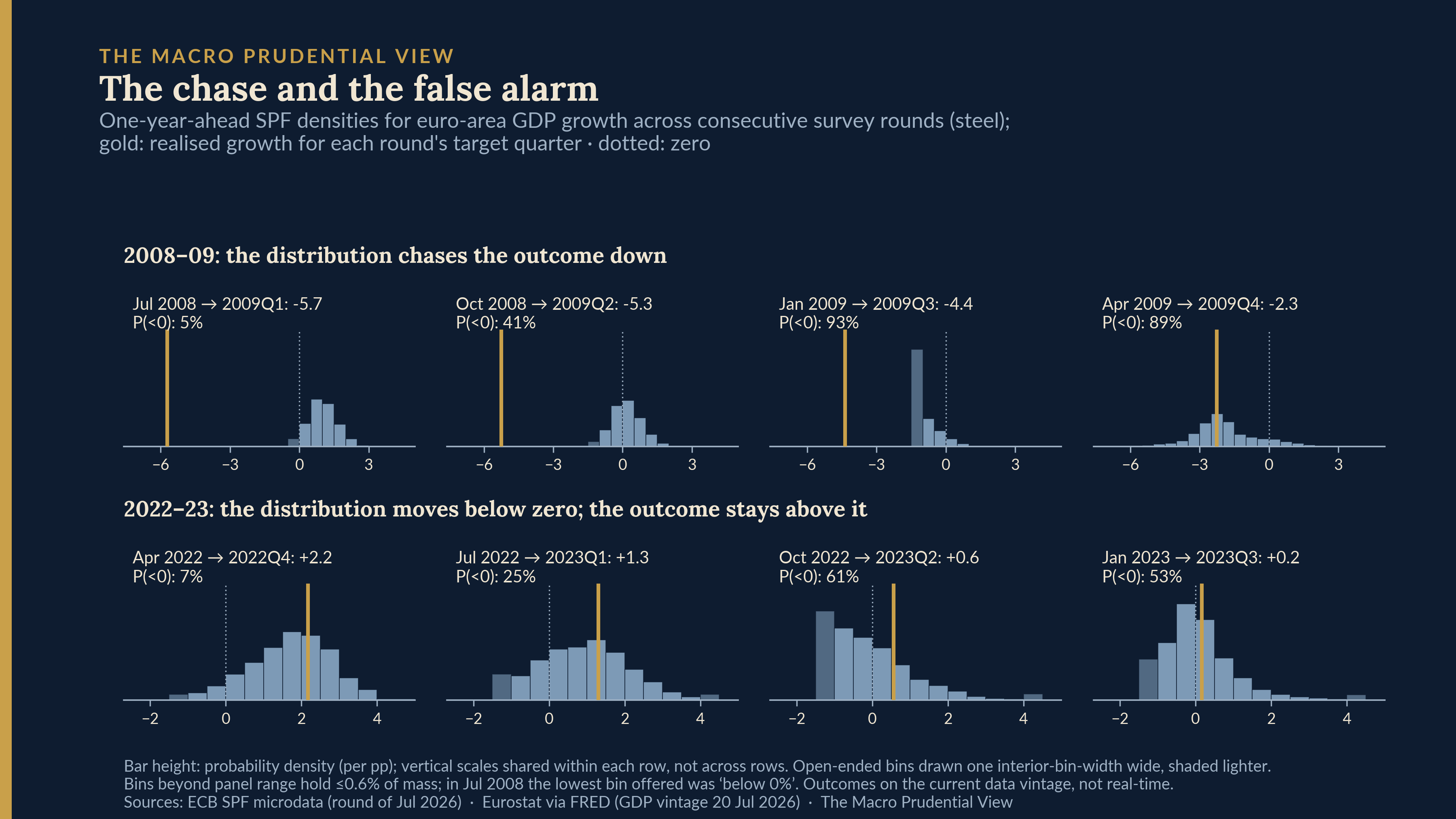
The two episodes compress the whole argument. In the top row the densities chase the outcome down, round after round, and the instrument itself limits what they could say: in July 2008 the lowest bin on offer was “below 0%”, so a respondent could express that a contraction might happen but not distinguish a mild one from the −5.7% that arrived. By January 2009 the panel had piled its mass into a spike near −1% while the year to 2009Q3 came in at −4.4% — direction finally right, depth still wrong. In the bottom row the mass walks below zero through the winter of 2022–23 while the outcome stays above it in every panel.
The panels invite a question the aggregate cannot answer: was early warning present in individual views and averaged away? The threshold decides the answer, so here is the sweep. Requiring the 90th percentile above 20% while the aggregate sits below 10%, the screen fires four times across 111 rounds, three resolved, and the only one followed by negative growth is October 2019 — the pandemic quarter, which no growth density plausibly foresaw. Lower the bar to 15% and July 2008 is caught, as it should be; but the same screen then fires twelve times, nine resolved, three followed by negative growth, two of those three again the pandemic. Lower it to 10% and four of fourteen resolved cases are followed by negative growth, three of them pandemic quarters. At that same threshold the upper decile crossed together with the aggregate in 2008 and in 2022, and one round earlier in 2011. July 2008 remains the sharpest exhibit: the median respondent attached zero probability to negative growth, the 90th-percentile respondent 15%, the most pessimistic 40%. The aggregate summarises that spread as 5% and does not publish the dispersion; no threshold in that range turns the dispersion into a rule: the cuts loose enough to catch 2008 also fire through years in which nothing followed. Other quantiles, trimmed or weighted aggregates, and panel-composition effects are not tested here. A fuller cross-sectional treatment, including threshold sensitivity, follows in Wednesday’s Note.
Mechanisms, and the Growth-at-Risk toolkit
Three mechanisms fit the record, at the strength the evidence allows. Aggregation: the equal-weight average is the ECB’s convention, not the only object one could build, and it compresses disagreement; in 2008, dispersion widened before the aggregate moved substantially, though on the screen above that pattern did not generalise into a rule, and whether alternative aggregations would have moved earlier is not tested here. Updating: a 5% ex-ante probability on an event that then occurs is not, in one draw, miscalibration; the late-arrival pattern rests on the two cyclical downturns, since the pandemic is not evidence either way; two episodes bound what a pattern can prove. The instrument: a fixed bin grid limits how finely severity can be expressed once probability mass reaches an open-ended tail bin, and the July 2008 grid is the exhibit.
The ESRB’s recent tail-risk work is the right reference point. Andersen et al. (2025) present a growth-at-risk model and the SPF density as complementary perspectives on euro-area downside risk — parallel lenses, not a weighted composite — and they note that the tighter survey distribution aligns with evidence that the SPF tends to underestimate the tails of the distribution, citing Clements (2011), Rich, Song and Tracy (2012) and the ECB’s own 25-year retrospective (Allayioti et al. 2024). On their own readings the two lenses diverged over 2025, the model’s 10th percentile falling to between −1.7% and −2.6% while the survey’s moved to about −0.4% — figures produced under their specifications and conditioning, not aligned here to a common origin and target.
The retrospective evaluates the densities with probability integral transforms. A PIT-based assessment asks whether realised outcomes are plausibly drawn from the forecast distribution over the full record; this piece asks a different question — whether the survey’s lower tail remained protective during the small number of persistent downturn episodes. The two exercises are complements, not competing verdicts. For instruments whose calibration, legal process and transmission require a horizon materially longer than the survey’s short-horizon information, the record here makes the aggregate density a weak candidate for a stand-alone tail-risk signal. Whether financial, market-based or balance-sheet indicators would have done better on the same dated information sets is not tested here — the comparison a user would most want, and the one this piece does not make. A lagging density that correctly identifies an economy already in a bad state retains monitoring value; the scope of this piece is ex-ante information for slow-moving tools. Whether any of this should change how such inputs are weighted inside a framework is a question for the framework’s owners, and outside this piece.
The current read
The Q3 2026 round expects growth of 0.6% this year, after a downward revision of 0.4 percentage points, and 1.2% in 2027. It attaches 5.4% to negative annual growth one year out and 5.1% at two years — a spread not worth interpreting. A 5.4% probability is low. The historical record assembled here provides no basis for treating a low survey probability as stand-alone reassurance, particularly for a user concerned with slow-building downside risk.
Across 1999–2026, then: the equal-weight aggregate SPF density scored better than two naive benchmarks, descriptively and by a margin not cleanly separated from zero, and repriced sharply as conditions deteriorated. But its record provides limited evidence that it identifies euro-area downturn tails early enough to stand alone for slow-moving macroprudential decisions. Its two-year tail barely opens; its lower-tail misses, on the current vintage, concentrate in the few persistent downturn episodes — though that small number of effectively independent episodes also prevents a decisive calibration verdict; and respondent disagreement, at every threshold tested here, does not supply a stable remedy.
Paweł Fiedor — The Macro Prudential View
Data described are as at 28 July 2026 (SPF round of July 2026, released 24 July; GDP vintage of 20 July 2026).
The author works at the Central Bank of Ireland and in the ESRB Secretariat. This piece is written in a personal capacity; views are the author’s own and should not be attributed to the Central Bank of Ireland, the ESRB, or the Eurosystem. It draws exclusively on publicly available sources and takes no position on whether the policy measures discussed should be adopted.
Method notes. ECB SPF individual-forecast microdata, 111 rounds, 1999Q1–2026Q3. Individual densities rescaled to sum to one where reported probabilities total between 90 and 110, otherwise dropped; equal-weight averaging across respondents (the ECB’s convention). Bin labels read as contiguous half-open intervals (upper label extended by 0.1pp); open-ended bins treated as one interior-bin-width wide for percentiles, means and density heights. Rolling targets identified by their gap from the round (roughly two and six quarters). Realised growth: euro area (EA20) chain-linked volumes, Eurostat via FRED, vintage 20 July 2026; outcomes evaluated on the current vintage except where real-time releases are cited. Exceedance interval: moving-block bootstrap, 8-quarter blocks, 10,000 draws; the interval is a resampling diagnostic rather than a confidence interval, and is stable across block lengths (4q: 11–36%; 6q: 10–37%; 12q: 11–38%; 16q: 11–37%). Dropping the two marginal breaches leaves 22 of 107 (20.6%); both sit inside larger clusters, so the episode pattern is unaffected. The GDP section of every round since 1999Q1 carries rolling one- and two-year targets alongside calendar-year questions — the 2008Q3 file, for instance, lists target periods 2008, 2009, 2010 and 2013 together with 2009Q1 and 2010Q1; the rolling densities are the object used here throughout, and the July 2008 round records 57 density responses for the year to 2009Q1. Percentiles are insensitive to the open-tail convention: the p10 falls inside the open bottom bin in 3 of 107 rounds, and the breach count is 24 of 107 whether that bin is assumed one, two, four or eight interior widths deep. Outcomes use the current-composition EA20 series; membership changed over the sample, so the geographical aggregate is not identical to the one every historical round forecast. The constant Brier benchmark uses the full-sample frequency and is therefore in-sample; the climatology benchmark uses only data available at each origin; excluding 2020–21 targets, the ranking is unchanged (survey 0.072, constant 0.099, climatology 0.111). The climatology benchmark starts once twelve quarters of history are available (first evaluated target 1999Q4). A paired block bootstrap on the survey-minus-climatology score differential gives a mean of −0.037 with a 95% interval of [−0.095, +0.005]: the survey is ahead in 95% of resamples, but the differential is not cleanly separated from zero, so the ranking is reported as descriptive. As a descriptive diagnostic only: excluding 2020–21, the mean of the aggregate density correlates 0.83 with annual growth over the year ending at the survey round and 0.67 with the growth it forecasts; overlapping annual windows induce persistence in both series, so these are raw cross-correlations, not a formal timing test. Cross-sectional statistics are computed over respondents with usable densities under the same rescaling rule; the panel ranges from 24 to 58 respondents per round at the one-year horizon, and changes in composition may contribute to measured dispersion. Derived series and scripts available on request.
Sources: ECB, Survey of Professional Forecasters — Q3 2026 report (24 July 2026) and individual-forecast microdata, 1999Q1–2026Q3 — https://www.ecb.europa.eu; Eurostat via FRED, euro area (EA20) real GDP, chain-linked volumes, series CLV10MNACB1GQSCAEA20Q, vintage 20 July 2026 — https://fred.stlouisfed.org; Eurostat, euro-indicators releases for 2023Q2 GDP: preliminary flash of 31 July 2023 (2-31072023-BP), flash of 16 August 2023 (2-16082023-AP) and estimate of 7 September 2023 (2-07092023-AP) — https://ec.europa.eu/eurostat; Andersen, F., M. Andersson, S. G. Cecchetti, R. Giuliana, U. Pelca, J. Rice, C. Sarchi and A. de Vries (2025), “Navigating Tail Risks: Assessing Euro Area Economic Growth and Equity Market Vulnerabilities”, Macroprudential Commentaries, Issue 9, European Systemic Risk Board, December, and the accompanying VoxEU column of 16 December 2025 — https://www.esrb.europa.eu, https://cepr.org; Allayioti, A., R. Arioli, C. Bates et al. (2024), “A look back at 25 years of the ECB SPF”, ECB Occasional Paper No 364; Clements, M. P. (2011), Journal of Money, Credit and Banking 43(1); Rich, R., J. Song and J. Tracy (2012), Federal Reserve Bank of New York Staff Report No 588; Adrian, T., N. Boyarchenko and D. Giannone (2019), “Vulnerable Growth”, American Economic Review 109(4). Chart data as cited in each figure.